
This is a repost of my feature on the Silectis blog.
With our Magpie platform, you can build a trusted data lake in the cloud as the shared foundation for analytics in your organization. Magpie brings together the tools data engineers and data scientists need to integrate data, explore it, and develop complex analytics.
For more information, reach out to me on my Contact Page or connect with me on LinkedIn.
The "gaps and islands" problem is a scenario in which you need to identify groups of continuous data (“islands”) and groups where the data is missing (“gaps”) across a particular sequence.
The problem may sound arcane at first glance but knowing how to solve this type of problem is critical for advanced SQL practitioners. These starting and stopping points in the data can represent significant business events, such as periods of peak sales activity, or can pinpoint missing data.
Unfortunately, figuring out where these boundaries occur can be one of the more complex SQL challenges that we face. The purpose of this post is to help you understand the characteristics of gaps and islands problems so that you will notice examples more often and be equipped to implement robust solutions.
Case Study
Gaps and islands appear in a variety of data sets and can take several forms. Sometimes, the sequence of interest is a numeric identifier (like those typical in relational databases) and solving for the gaps means finding the records in the sequence which were deleted. The techniques described below can be invaluable for troubleshooting third-party data and can enable advanced use cases like data completeness checks within an ETL pipeline.
The problem formulation may also arise when dealing with temporal data, for example in cases where it is useful to decipher periods of activity or inactivity. Most notably, identifying “islands” is a critical step for transforming event-level data into historized data warehouse models such as slowly changing dimensions.
Let’s take a look at an example.
Deciphering Boundaries Using Ranking Functions
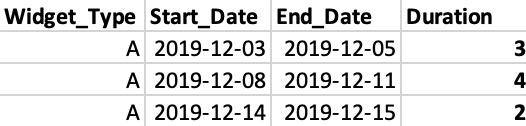
Imagine that your company manufactures several types of widgets. Unfortunately, one of the production lines has mechanical problems that force the line manager to reduce output of Widget A. As an analyst, you want to determine how long it takes the production line to get back to full capacity during each of these episodes.
The company logs this production line as having downtime if it produces less than 20 units/day. Here we see three “islands” of continuous data in which the production line experiences downtime.
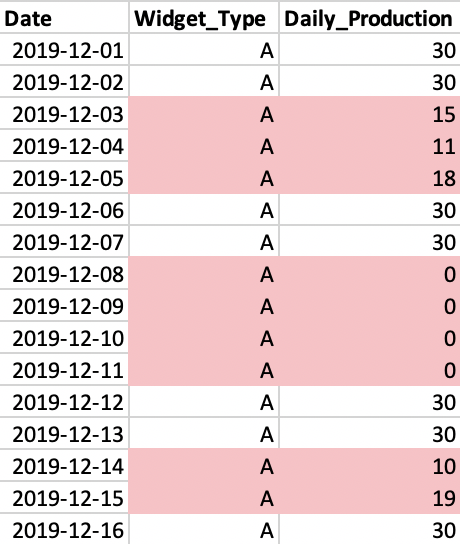
Structuring this question in SQL is a bit tricky. We’re not interested in the total number of days showing downtime, which could be found via a simple COUNT(). We want to determine the duration required to restore the production line to its full capacity, as measured from the start of downtime. In the above example, we should be able to calculate three, four, and two days for each outage, respectively.
Let’s take a look at how I structured the query:
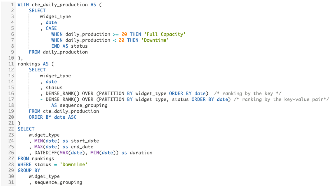
The first common table expression selects the widget type, the date, and derives a “status” column based on the daily production.
The second common table expression is the crux of the problem. We derive the “islands” by comparing the output of two DENSE_RANK() functions, which acts as an indicator for when the data switches from one island to another.
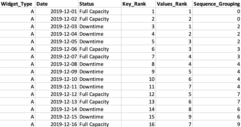
Diving into this step, the “rankings” query can be visualized using the table above. The first DENSE_RANK() function (“Key_Rank” in the table) computes the ranking for records of Widget A, ordered by date in ascending order. Since we’re only looking at Widget A in this example, Key_Rank is monotonically increasing for the range.
The second DENSE_RANK() function (“Values_Rank” in the table) ranks according to Widget Type + Status, in this case behaving like two running counters (one for each of the statuses). Note: SQL’s LEAD(), LAG(), and ROW_NUMBER() functions can also be used to generate the desired groupings. However, they are more more sensitive to duplicate data, so I prefer to use DENSE_RANK().
Sequence_Grouping is the difference between the ranking functions and is a constant value for all records in the same “island”.
Finally, the concluding query calculates the start date, end date, and duration of downtime periods. We’re able to do so by virtue of the values of the derived “Sequence_Grouping” field, which allow us to utilize a GROUP BY statement.
The output of the overall query returns the desired information and the SQL is in form that can be generalized for analyzing other production lines as well.
Building a Slowly Changing Dimension from Historical Data
Knowing how to transform data in this way unlocks new capabilities. Continuing with the same hypothetical company, imagine you’re interested in analyzing the daily production goals for each type of widget. From a data warehousing perspective, it would be quite useful to compare sales performance for each widget against the corresponding production goal(s) for the same time period. The appropriate way to model this is as a slowly changing dimension.
Generally, the daily production goals are static, but occasionally inventory issues or changes in customer demand cause a goal to be adjusted. Unfortunately, the production goals are set by the warehouse manager in a legacy system and we’re only able to get a monthly data dump at a daily granularity.
This is what the data looks like for three particular widgets.
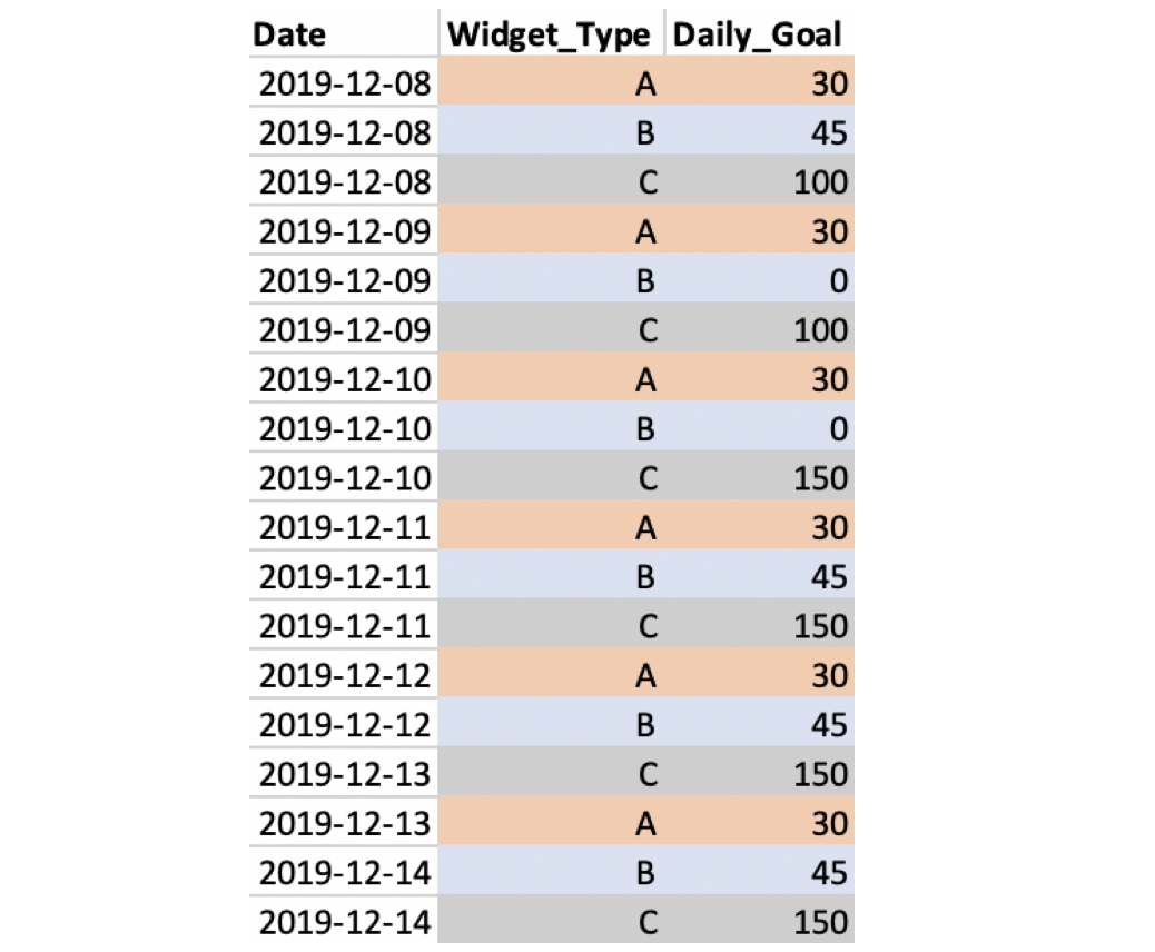
Widget A had a constant goal of 30 units per day. Widget B had a daily production goal of 45 widgets but didn’t produce on December 9th and 10th due to planned maintenance. It resumed it previous goal on the 12th. Widget C targeted 100 units per day, but on December 10th, the warehouse manager increased the daily goal due to increased customer demand.
To restructure the data, let’s create a table using the same ranking strategy shown above. Instead of “start_date” and “end_date”, we name the equivalent fields “valid_from” and “valid_to”.
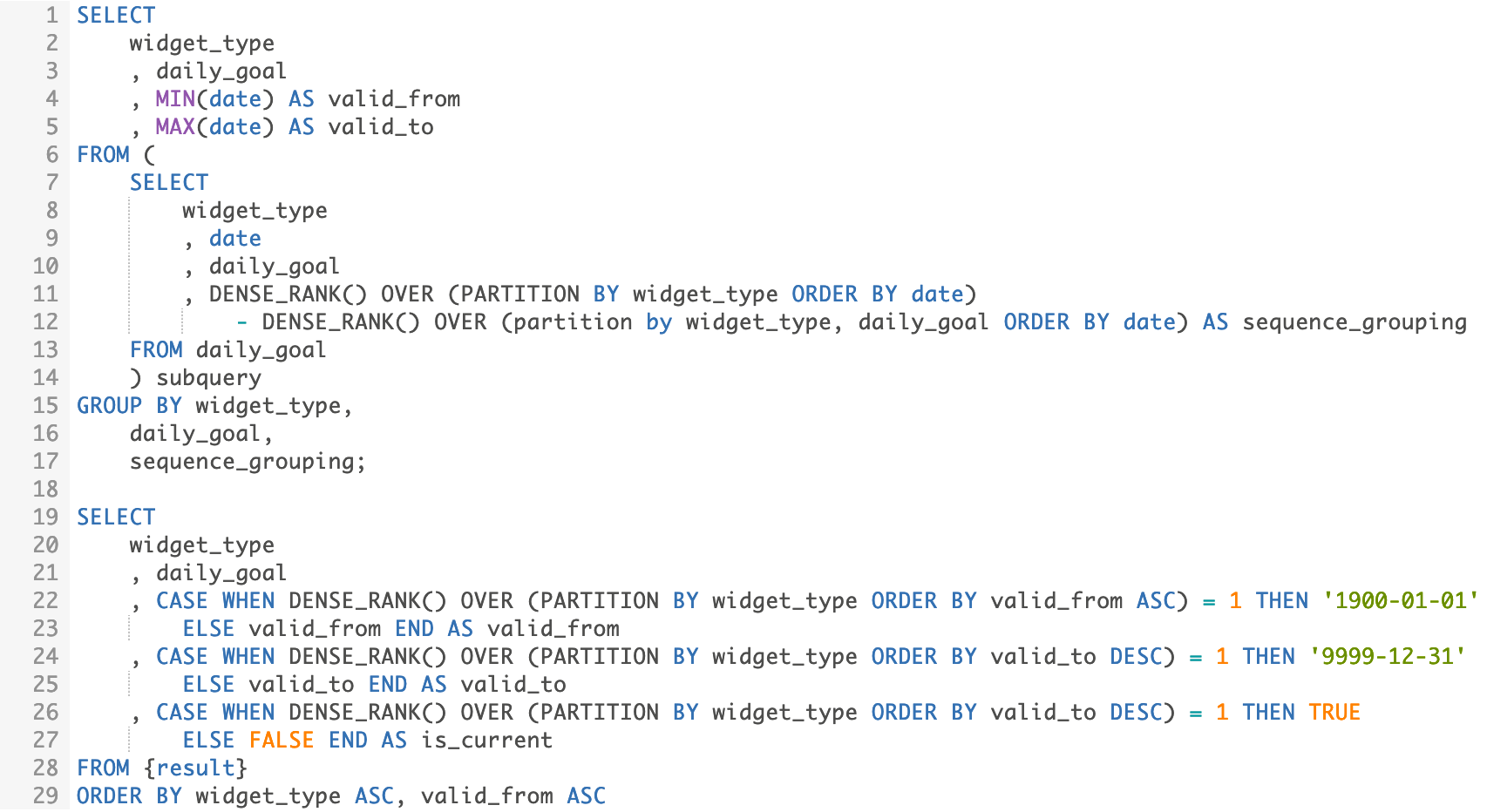
The output of this query will be very similar to the output from the first example, but we’re not quite done yet. Analysts frequently use range queries to return records for a specified time period. We want to adjust the first “valid_from” to be a date in the far past and the last “valid_to” to the far future to ensure queries behave appropriately.
To complete the dimension table, we also add an “is_current” flag. This indicator is useful for reporting on the most recent version of the daily goal for each widget.
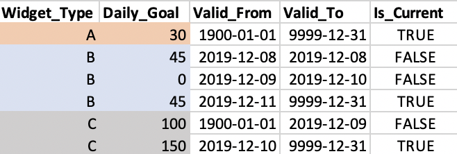
The table above shows the dimension table for Widgets A, B, and C. Note that new records are included for every change to the daily goal for a widget, and the prior record is invalidated.
Conclusion
In this post, we explored advanced techniques that can help you generate new insights and transform existing data into useful models. Hopefully you’ve been able to expand your SQL toolkit and feel ready to tackle your own data challenges.
If your organization wants to set up advanced data pipelines without the hassle of managing infrastructure, click here to see how Magpie can help.
Matt Boegner is a Data Engineer at Silectis.
You can find him on LinkedIn.